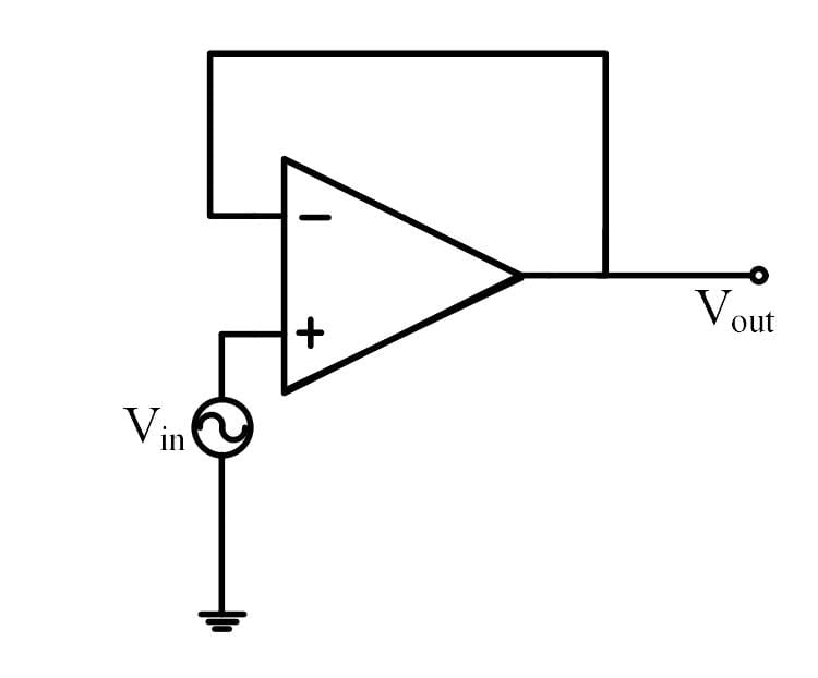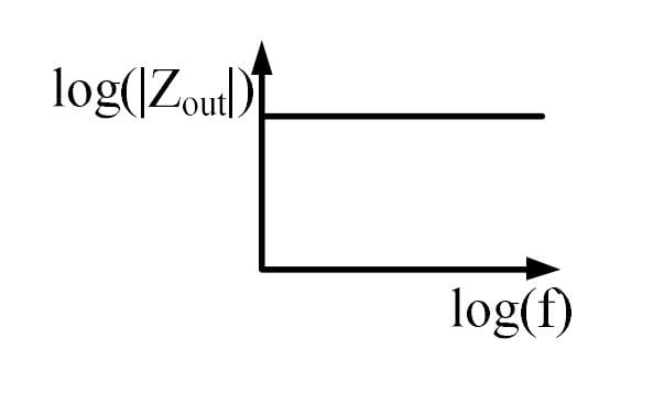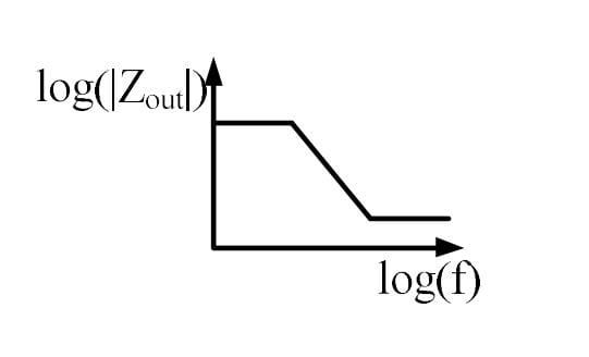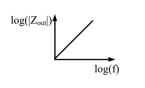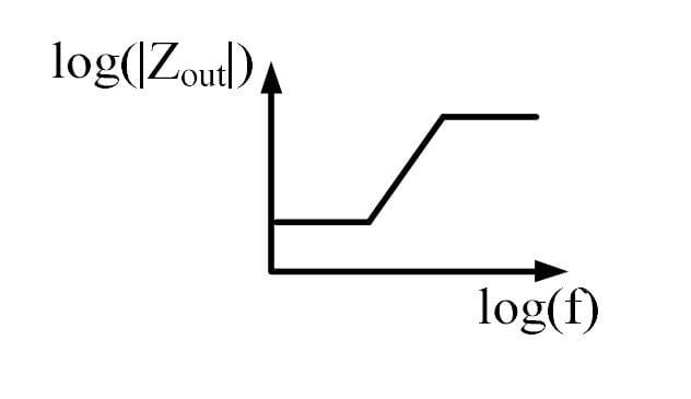
The output impedance of a non-ideal operational amplifier is denoted by Z_out . The variation in the magnitude of Z_out with increasing frequency, f , in the circuit shown below, is best represented by

Correct Answer: The variation of $\left|Z_{\text{out}}\right|$ with frequency $f$ is best represented by the curve in the option containing the graph that starts flat at a lower value, increases with a constant slope at intermediate frequencies, and then flattens out again at a higher value (corresponding to the image: WhatsApp Image 2024-09-30 at 2-1727688854245.jpeg).

Explanation and Step-by-Step Derivation:

1. Understanding the Circuit Configuration
The provided circuit diagram shows a non-inverting operational amplifier with its output terminal connected directly back to its inverting input terminal ($-$). The input voltage $V_{\text{in}}$ is applied to the non-inverting terminal ($+$). This configuration represents a negative feedback system known as a unity-gain buffer (or voltage follower). For this configuration, the feedback factor is:
$\beta =1$

2. Formula for Closed-Loop Output Impedance
In a negative feedback amplifier, negative feedback reduces the output impedance. The closed-loop output impedance $Z_{\text{out}}$ is related to the open-loop output resistance $R_o$ and the open-loop gain $A\left(f\right)$ by the relation:
$Z_{\text{out}}\left(f\right)=\frac{R_o}{1+A\left(f\right)\beta }$
Since $\beta =1$, this simplifies to:
$Z_{\text{out}}\left(f\right)=\frac{R_o}{1+A\left(f\right)}$

3. Modeling the Frequency Dependence of the Open-Loop Gain
A practical, internally compensated operational amplifier has an open-loop gain that rolls off at high frequencies. This behavior is typically modeled as a single-pole low-pass transfer function:
$A\left(f\right)=\frac{A_0}{1+j\frac{f}{f_c}}$
where $A_0$ is the DC open-loop gain (which is very large, typically in the range of ${10}^5$ to ${10}^6$) and $f_c$ is the open-loop corner (cutoff) frequency (typically around $10\text{Hz}$).

4. Deriving the Closed-Loop Output Impedance
Substitute the expression for $A\left(f\right)$ into the output impedance formula:
$Z_{\text{out}}\left(f\right)=\frac{R_o}{1+\frac{A_0}{1+j\frac{f}{f_c}}}$

5. Analysis of Frequency Regions
To determine the shape of the magnitude graph in a log-log plot (i.e., $log\left(\right|Z_{\text{out}}\left|\right)$ versus $log\left(f\right)$), we evaluate three distinct frequency ranges:

Case I: Low Frequencies ($f\ll f_c$)
Here, the frequency term is extremely small compared to $1$, so $j\frac{f}{f_c}$. The output impedance becomes:
$Z_{\text{out}}\approx \frac{R_o}{1+A_0}$
Since $A_0$ is a constant value, the output impedance is constant and independent of frequency in this region. This corresponds to the flat plateau at low frequencies.

Case II: Intermediate Frequencies ($f_c\ll f\ll A_0{f}_c$)
In this region, the frequency $f$ is much larger than the corner frequency $f_c$, meaning $\frac{f}{f_c}$, so the numerator's imaginary term dominates over 1. However, $\frac{f}{f_c}$ is still significantly smaller than the open-loop gain $A_0$, so the denominator is dominated by $A_0$:
$Z_{\text{out}}\approx R_o\left(\frac{j\frac{f}{f_c}}{A_0}\right)$
Taking the magnitude of both sides:
$\left|Z_{\text{out}}\right|\approx \left(\frac{R_o}{A_0{f}_c}\right)f$
Taking the logarithm:
$log\left(\right|Z_{\text{out}}\left|\right)\approx log\left(f\right)+log\left(\frac{R_o}{A_0{f}_c}\right)$
This represents a straight line with a slope of $+1$ (equivalent to $+20\text{dB/decade}$). Thus, the magnitude of output impedance increases linearly with frequency in this range.

Case III: High Frequencies ($f\gg A_0{f}_c$)
At very high frequencies, the term $\frac{f}{f_c}$ becomes much larger than both 1 and $A_0$. The imaginary terms dominate in both the numerator and the denominator, leading to:
$Z_{\text{out}}\approx R_o\left(\frac{j\frac{f}{f_c}}{j\frac{f}{f_c}}\right)=R_o$
Thus, the magnitude of the output impedance levels off at a constant value equal to the open-loop output resistance $R_o$, resulting in another flat horizontal region at a higher impedance value.

Conclusion
Combining the three regions, the log-log plot of $\left|Z_{\text{out}}\right|$ vs frequency $f$ begins flat at a low impedance level ($\frac{R_o}{1+A_0}$), increases linearly with a slope of $+1$ at intermediate frequencies, and then flattens out at a higher value ($R_o$). This is accurately depicted in the plot shown in the fourth option.